

#13 PCA

PCA (Principal Component Analysis) is a dimensionality reduction technique and helps us to reduce the number of features in a dataset while keeping the most important information. It changes complex datasets by transforming correlated features into a smaller set of uncorrelated components.
What is PCA?
Principal Component Analysis (PCA) is an unsupervised machine learning algorithm used for:
Dimensionality reduction
Feature extraction
Data compression
Noise reduction
Data visualization
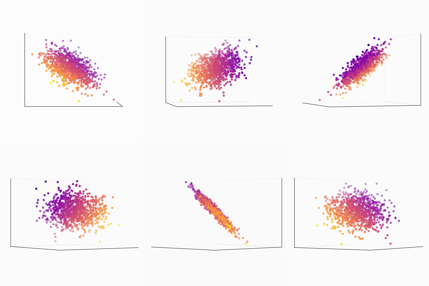
PCA transforms high-dimensional data into fewer dimensions while preserving most of the important information.
Why PCA is Needed
Sometimes datasets contain:
Too many features
Redundant information
Correlated variables
PCA helps by reducing the number of features while keeping maximum variance.
Real-Life Example
Suppose a student dataset contains:
Math marks
Physics marks
Chemistry marks
Biology marks
Most marks may be correlated.
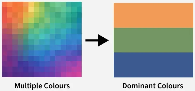
PCA combines them into fewer important components.
What is Dimensionality Reduction?
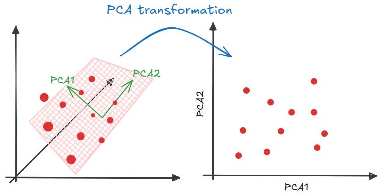
Reducing N dim -> K dim
where N = original features, K = reduced features
Example : 100 features→2 principal components
Key Idea of PCA
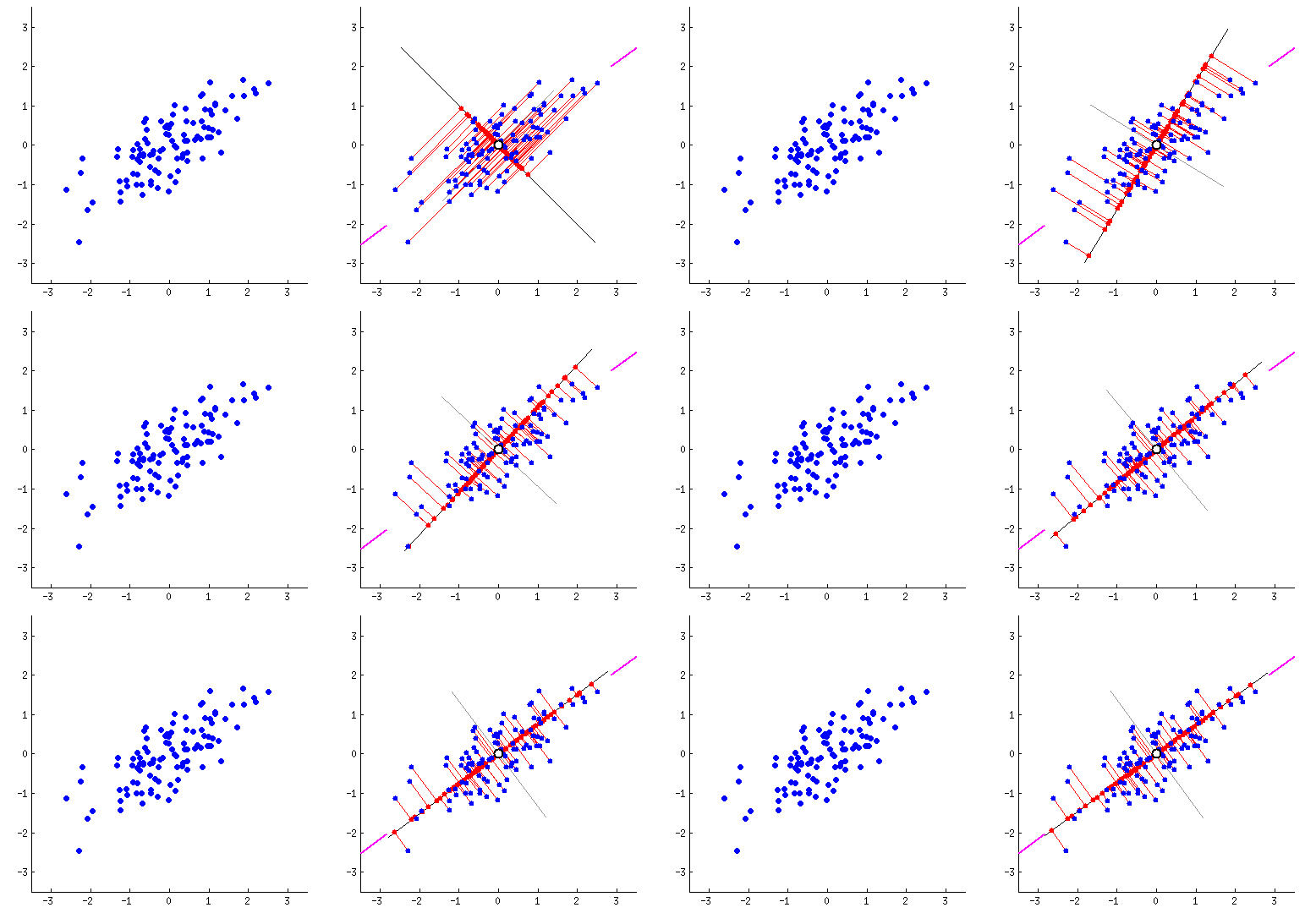
PCA finds new axes called Principal Components.
These Components - Capture maximum variance, are perpendicular to each other, reduce redundancy.
Principal Components
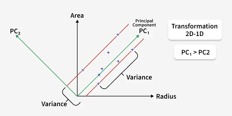
First Principle Component (PC1)
Captures maximum variance.
Second Principle Component (PC2)
Captures Second highest variance.
and so on....
PCA Workflow
Step 1 — Standardize Data
Since features may have different scales, PCA first standardizes data.
$$\mathbf{z = \frac{x - \mu}{\sigma}}$$
| Symbol | Meaning |
|---|---|
| (x) | Data point |
| mu | Mean |
| sigma | Standard deviation |
Step 2 — Calculate Mean
Mean formula
$$\mathbf{\mu = \frac{\sum x}{n}}$$
Step 3 — Compute Covariance Matrix
Covariance measures how two variables vary together.
$$\mathbf{Cov(X,Y)=\frac{\sum (X-\bar{X})(Y-\bar{Y})}{n-1}}$$
Covariance matrix - for 2 features

Step 4 — Find Eigenvalues and Eigenvectors
PCA calculates eigenvalues and eigenvectors from the covariance matrix.
Eigenvalue Equation
$$\mathbf{Av = \lambda v}$$
| Symbol | Meaning |
|---|---|
| (A) | Covariance matrix |
| (v) | Eigenvector |
| (\lambda) | Eigenvalue |
What are Eigenvectors?
Eigenvectors represent the directions of maximum variance.
What are Eigenvalues?
Eigenvalues represent the amount of variance captured.
Higher eigenvalue means:
more important component
more information retained
Step 5 — Select Principal Components
Choose components with highest eigenvalues.
Example:
$$\mathbf{\lambda_1 > \lambda_2 > \lambda_3}$$
Select PC1, PC2
Step 6 — Transform the Data
Project original data onto principal components.
Projection Formula
$$\mathbf{Z = XW}$$
| Symbol | Meaning |
|---|---|
| X | Original data |
| W | Eigenvector matrix |
| Z | Transformed data |
Variance in PCA
PCA tries to maximize variance.
Variance Formula
$$\mathbf{Var(X)=\frac{\sum (X-\bar{X})^2}{n}}$$
Higher variance means : More information, better feature represenatation.
Explained Variance Ratio
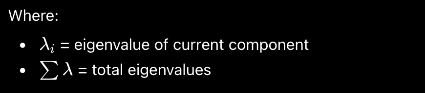
Measures how much information each principal component preserves.
Formula:
$$\mathbf{ Explained \ Variance =\frac{\lambda_i}{\sum \lambda} }$$
Simple PCA Example with Dataset
Dataset:
| Student | Math ((X)) | Physics ((Y)) |
|---|---|---|
| A | 2 | 3 |
| B | 4 | 5 |
| C | 6 | 7 |
We will reduce : 2D -> 1D using PCA
Step 1 — Calculate Mean
Mean of X
$$\mathbf{ \bar{X} =\frac{2+4+6}{3} } =4$$
Mean of Y
$$\mathbf{ \bar{Y} =\frac{3+5+7}{3} } =5$$
Step 2 — Standardize Data
Formula:
$$\mathbf{ z=\frac{x-\mu}{\sigma} }$$
For simplicity, we center data by subtracting means.
Centered data
| Student | X- X_bar | Y - Y_bar |
|---|---|---|
| A | (2 - 4 = -2) | (3 - 5 = -2) |
| B | (4 - 4 = 0) | (5 - 5 = 0) |
| C | (6 - 4 = 2) | (7 - 5 = 2) |
Step 3 — Covariance Matrix
$$\mathbf{ Cov(X,X) =\frac{ (-2)^2+0^2+2^2 }{2} }$$
$$={\frac{4+0+4}{2} =4 }$$
$$\mathbf{ Cov(Y,Y) =\frac{ (-2)^2+0^2+2^2 }{2} } =4$$
$$\mathbf{ Cov(X,Y) =\frac{ (-2)(-2)+(0)(0)+(2)(2) }{2} }$$
$${=\frac{4+0+4}{2} =4 }$$
there fore covariance matrix :

Step 4 — Find Eigenvalues

Determinant Calculation
$$\mathbf{ (4-\lambda)(4-\lambda)-16=0 }$$
$$\mathbf{ (4-\lambda)^2-16=0 }$$
$$\mathbf{ 16-8\lambda+\lambda^2-16=0 }$$
$$\mathbf{ \lambda^2-8\lambda=0 }$$
Eigenvalues
$$\mathbf{ \lambda_1=8 }, \mathbf{ \lambda_2=0 }$$
Largest Eigenvalue :
$$\mathbf{ \lambda_1=8 }$$
So, PC1 is selected
Step 5 — Find Eigenvector
formula
$$\mathbf{ (C-\lambda I)v=0 }$$
Substitute:

Equation:

$$\mathbf{ -4x+4y=0 }$$
$$\mathbf{ x=y }$$
Eigenvector:

Step 6 — Final Principal Component
Principle component

This direction captures maximum variance.
Final Reduced Data
Original
$$\mathbf{ (X,Y) }$$
Reduced
$$\mathbf{ PC_1 }$$
So PCA successfully reduces :
$$\mathbf{ 2D \rightarrow 1D }$$
Advantages of PCA
Reduces dimensionality
Faster model training
Removes redundancy
Helps visualization
Reduces overfitting
Compresses data
Disadvantages of PCA
Information loss can occur
Hard to interpret components
Sensitive to scaling
Works best for linear data
Applications of PCA
Face recognition
Image compression
Data visualization
Noise filtering
Feature engineering
Bioinformatics
PCA vs Feature Selection
| PCA | Feature Selection |
|---|---|
| Creates new features | Selects existing features |
| Uses transformations | Keeps original columns |
| Reduces dimensions | Removes unnecessary features |
Python Code
from sklearn.decomposition import PCA
import numpy as np

# Original Dataset
X = np.array([
    [2, 3],
    [4, 5],
    [6, 7]
])

print("Original Dataset:\n")
print(X)

# Create PCA Model

pca = PCA(n_components=1)

# Apply PCA

X_pca = pca.fit_transform(X)

# Outputs

print("\nReduced Data:")
print(X_pca)

print("\nPrincipal Component:")
print(pca.components_)

print("\nExplained Variance:")
print(pca.explained_variance_)

print("\nExplained Variance Ratio:")
print(pca.explained_variance_ratio_)
Curse of Dimensionality
The Curse of Dimensionality refers to the problems that arise when the number of features (dimensions) in a dataset becomes very large.
As dimensions increase:
Data points become sparse.
Distance calculations become less meaningful.
More training data is required.
Model complexity increases.
Computational cost becomes higher.
Example
Suppose we have a dataset with only 2 features. Data points may be densely packed and patterns are easy to find.
If the dataset has 1000 features, the data becomes highly sparse and points appear far apart from each other, making learning difficult.
Why PCA Helps
PCA reduces the number of dimensions while preserving most of the important information, helping to overcome the curse of dimensionality.
Sparse Features and Sparse Datasets
What are Sparse Features?
A feature is called sparse when most of its values are zero or empty.
Example
| User | Movie A | Movie B | Movie C |
|---|---|---|---|
| U1 | 5 | 0 | 0 |
| U2 | 0 | 4 | 0 |
| U3 | 0 | 0 | 5 |
Most entries are zero, so the dataset is sparse.
Common Problems with Sparse Datasets
Increased memory usage
Slower training
Difficult pattern discovery
Poor distance calculations
Higher risk of overfitting
Why Machine Learning is Difficult with Sparse Features
When most feature values are zero, data points become very different from each other. Similarity measures such as Euclidean distance become less reliable, making clustering and classification more difficult.
Ways of Dealing with Sparse Features
Feature Selection – Remove irrelevant features.
PCA (Principal Component Analysis) – Reduce dimensionality.
Feature Extraction – Create new informative features.
Remove Rare Features – Discard features that occur very infrequently.
Regularization – Reduce model complexity.
Use Sparse Data Structures – Store only non-zero values efficiently.
These techniques help improve model performance and reduce computational cost.
Sparse Data vs Missing Data
Although they may look similar, sparse data and missing data are different.
| Sparse Data | Missing Data |
|---|---|
| Value exists and is usually zero. | Value is unknown or unavailable. |
| Represents absence of an event or feature. | Represents unavailable information. |
| Common in text mining and recommendation systems. | Common in surveys and real-world datasets. |
| Example: User did not watch a movie → 0 | Example: User rating not recorded → NULL |
Example
Sparse Data:
User | Movie A |
U1 | 0 |
Here, 0 means the user did not watch the movie.
Missing Data:
User | Movie A |
U1 | NULL |
Here, NULL means the information is unavailable.
Key Difference
Sparse Data: The value is known and usually zero.
Missing Data: The value is unknown or not recorded.
Conclusion
PCA is a powerful dimensionality reduction technique that transforms high-dimensional data into fewer meaningful components while preserving maximum variance. It helps simplify datasets, improve computational efficiency, reduce redundancy, and visualize complex data effectively.


